|
|
|
|
|
|
|
|
|
|
When you click
Numerical model data can be animated, zoomed in and out, viewed in Plan View, Cross Section, Time Height, and Sounding; and loaded using line contours or color contours (images).
When you
select a model "family", you are selecting a predetermined set of 8 model
products. For example, when you select ![]() and then ETA40 family, FX-Net loads the following
products automatically:
and then ETA40 family, FX-Net loads the following
products automatically:
 |
FX-Net will automatically select the correct number of frames for each model family to get you all the times from the latest run. For example, selecting ETA40 under **Families** will automatically load 17 frames (0-48 hours; every 3 hours); selecting GFS will load 24 frames.
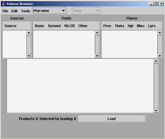
The Volume Browser
| When
you select Browser from the FX-Net Volume menu, the
Volume
Browser appears. This is the window from which you will
tailor and load whatever numerical model data you need to analyze.
The menu bar along the top of the volume browser is similar to the
main menu bar. In File, you may
exit the volume browser. In Edit, you may clear your
choices of Sources, Fields,
Planes, clear all choices, or select all or
none of your choices. In Tools, there are choices of
Baselines (used in loading cross sections), and Points
(used in loading time-height forecasts). Clicking Plan
View will open a menu with choices of how you want to view the
data, e.g. Plan View, Cross Section, Time Height or Sounding.
Below the menu bar are three smaller windows for choosing Sources (different numerical models), Fields (500mb height, MSLP, temperature, thickness, etc), and Planes (500mb level, 300K surface, 1500 meters, 1000-500mb layer, etc.). When you have chosen a Source, Field and a Plane that FX-Net is capable of loading, the product will appear in the Products window below the three smaller windows. If you have chosen a configuration that can't be loaded, such as a Field that the model doesn't have, or a Plane that the Field doesn't apply to, the product will simply not appear in the Products window. Some of the numerical models included in FX-Net at this time are the GFS, Eta (NAM), NGM, RUC, ECMWF, UKMET,and the WRF/Chem model. |
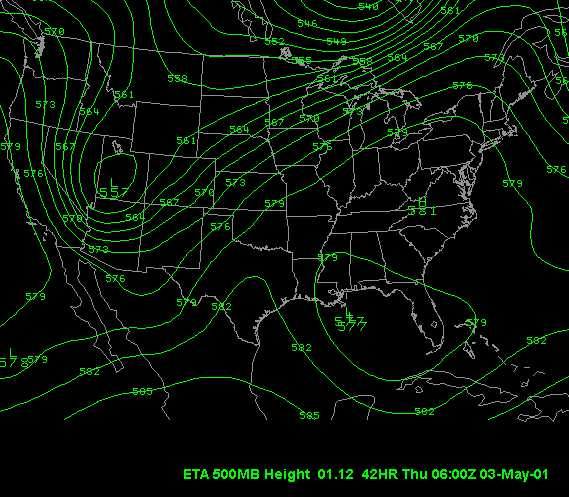
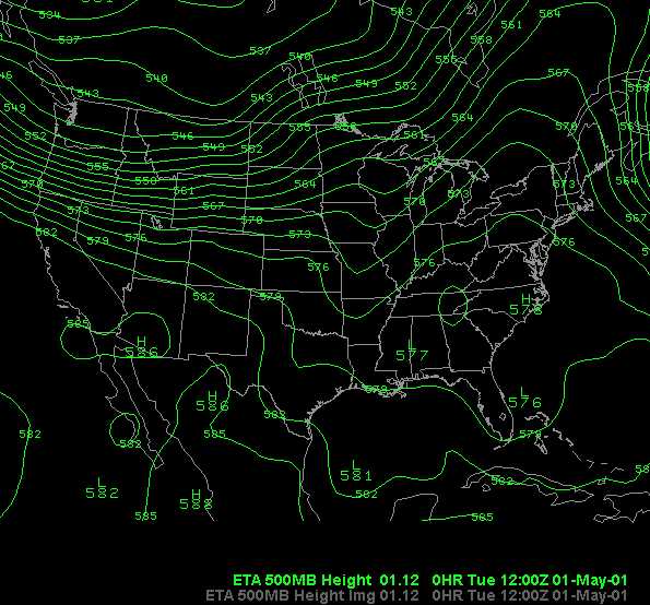
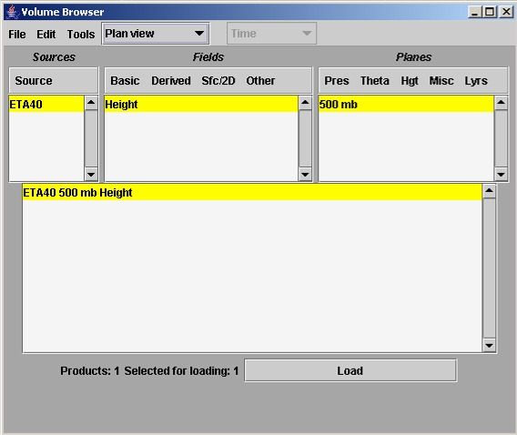
| Let's
jump right in and load a loop of ETA 500 mb heights into the primary
window. First, I choose how many frames I want to load.
The Eta40 run has 48 hours available, so 17 frames would be enough
to get all 48 hours in 3-hour increments. I chose 17 frames
from the main toolbar. Now I make sure that the map scale
(CONUS, Regional, N. Hemisphere, etc.) applies to the model selected.
Now I click Volume, then Browser and my volume browser
opens up. I am in Plan View, which is how to view 500
Mb heights. I click Source, then ETA40, then
under Fields choose Basic, then Height.
Finally, I choose Pres under Planes, and select
500mb. Once I do this, ETA40 500 Mb Height appears
in the Product window below. Your volume browser should now
appear exactly
like this.
To load the product, just select Load and it will load in the primary window. Once it is finished loading, you may create another loop to overlay in the primary window. Remember that only 8 products will load in the primary window, only one being an image product type. New with version 3.2 is the capability of increasing the density of numerical model contour data. You can do this two ways. First, you can simply load the data per instructions above, and use the Global Density on the toolbar to increase/decrease the number of contours. This changes the density of ALL products in the primary window. Second, now with version 3.41 you can also change the density of individual products in the primary window. After they are loaded, right-click the product title in the bottom right of the primary window that you want to change, and you select Set Density. A lesson on this is located here. |
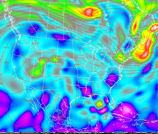
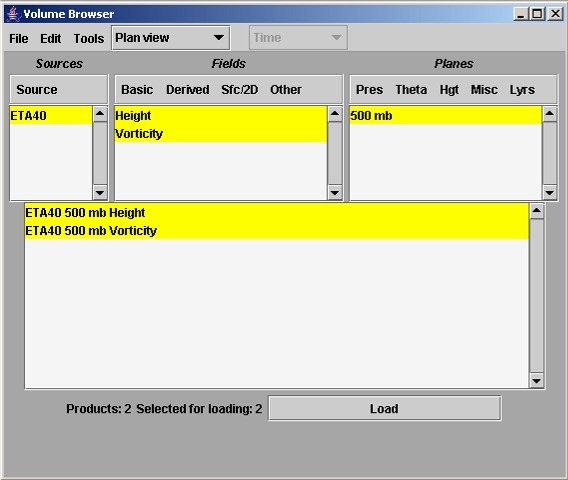
| In
addition to loading model data with the volume browser in contoured
format, most data can be loaded in image format. So as an example,
I now want to load the vorticity image (not contour
lines) at 500 Mb into the primary window, overlaying the 500 Mb heights
already there. I select Derived
under Fields, then Vorticity. Immediately the
ETA40 500 Mb Vorticity title appears in the bottom product
window. This is because I already had ETA40 under Sources
and 500mb under Planes chosen. My volume
browser now appears like
this image. It says that there are 2 products selected for
loading (on the bottom left), and I already loaded the 500 Mb heights,
so I de-select it by either clicking on Height under Fields,
or on ETA 500 Mb Height in the bottom Products window.
Next, if I right-click on the ETA 500 Mb Vorticity which is highlighted in the bottom product window, I see a small window pop up:
Now
I just select ETA 500 Mb Vorticity Image and I see the highlighted
product change to:
Then I click Load and the ETA 500 Mb Vorticity Image loads with the ETA 500 Mb Height in the primary window. |
Keep in mind that image-type data takes longer to load than contour-type data. Also, while it can be useful to view some fields as images, such as Vorticity, some fields, such as Heights, are not so well represented as images. It is personal preference, so experiment with the fields to see which you prefer as images.
Now that you are basically familiar with the volume browser and loading loops of numerical model data, let's look at the volume browser in more detail.
What is available in the Source menu depends on what map scale you chose from the FX-Net toolbar before you opened the volume browser. For example, the RUC is not available when the map scale is N. Hemisphere in the primary window. This is because the RUC is more of a mesoscale model and doesn't extend it's domain that far. The map in the primary window would have to be North American or smaller scale for the RUC to be available. To choose a model, simply click Source and then the model you want when the menu opens. If the model you want to use is not present when you open the volume browser and click Source, then close the volume browser and change the map scale in the primary window using the tool bar.
There are four ways to view numerical model data using the volume browser. These were mentioned above and are Plan View, Cross Section, Time Height and Sounding. Choosing one of these will give you different menus under Fields and Planes.
You can view the different menus in Plan View, Cross Section, Time Height and Sounding below, by moving your mouse cursor over the menu titles under Sources, Fields and Planes.
| Plan View | 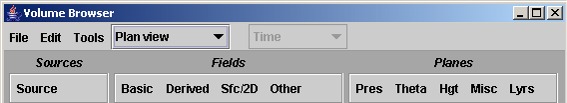 |
| Cross Section |  |
| Time Height | 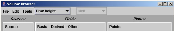 |
| Sounding | 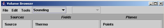 |
As
you can see, the Source menu under each is the same. The Fields
menu for Sounding has only one sub-menu, Thermo. The Basic,
Derived and Other menus remain present for the top 3 views,
with a Sfc/2D menu added to the Plan View Fields
section.
The menus specific to plan view are Sfc/2D under Fields, and all five Planes menus. Plan View is basically a bird's-eye view of data that is plotted on a horizontal or pseudo-horizontal map. It is the most common type of view when viewing meteorological data.
The Sfc/2D menu has extra fields that are usually only plotted at the surface. They include Precipitation, 6 and 24-hour Precipitation, Precipitable Water, Lifted Index, CAPE, CIN, Helicity, Mixing Ratio and Fire Index. If you choose any Field from the Sfc/2D menu, be sure to choose Surface from the Misc menu under Planes. Sometimes this is done automatically, and others you have to specify Surface.
The Planes menus in Plan View are fairly straightforward. The Pres menu contains options at various pressure levels in the atmosphere (250 Mb, 500 Mb, etc.). The Theta menu has many different Theta surfaces (300K, 310K) to choose from to plot your data. Using the Hgt menu, you may plot your data at a specific height, for example, 1500 meters. Finally, the Misc menu has choices like Surface, BL (boundary layer), and various layers (1000-500mb, 850-500mb, etc.).
To
load numerical model data using Plan View, follow the steps above,
where we loaded ETA 500MB Heights and ETA 500MB Vorticity Image.